Digital Approaches for the Synthesis of Poorly Accessible Biodiversity Information
Genomes for BacDive strains
As part of the DiASPora project, genomes from various ressources were associated to BacDive strains. This was necessary to provide the basis for genome-based predictions, as they will be developed in WP 3 and WP 4.
The matching is based on culture collection numbers and NCBI Taxonomy-IDs. A validation step uses species names and all of their known basonyms to verify the correctness of the matching procedure.
Result
We were able to associate almost 255,000 genomes from NCBI, PATRIC, and IMG to almost 10,000 BacDive strains. The following table gives an overview on all the data that were gained in this process. Beforehand, only 1,333 BacDive strains had genome associations, signifying a 7.5-fold increase. It is noticable that almost two-thirds of all bacterial type strains have a sequenced genome (If you do not know what a type strain is, read more here).
| Data type | Number of entries |
|---|---|
| Genomes from all ressources | 254,966 |
| Genomes from NCBI | 112,799 |
| Genomes from PATRIC | 136,863 |
| Genomes from IMG | 5,304 |
| Strains with genomes | 9,970 |
| Complete genomes | 18,477 |
| Strains with complete genome | 2,738 |
| Type strains in BacDive | 14,091 |
| Type strains with genome | 8,823 |
Genome-based predictions
The BacDive database was exploited to train artificial intelligence and subsequently complemented with genome-derived predictions.
Currently [Feb 2023], the BacDive database covers more than 19,000 type strains. More than 72 % of them have a genome sequence available. However, the coverage of phenotypic traits varies highly depending on the type of trait. While the growth temperature is required for successful cultivation and covered for most strains, the coverage of traits that are more difficult to access is low (figure 1). A good example is Gram straining, a method developed by Hans Gram in 1884: even though this is a standard test, it is only covered for 28 % of all type strains with genomes.

As part of the DiASPora project, BacDive datasets were exploited to train artificial intelligence and subsequently complement the database with genome-derived phenotypic traits. Therefore, we used known phenotypic traits from the database as labels to feed a Support Vector Machine (SVM). The model was trained to predict phenotypes based on Protein family (Pfam) annotations of the respective genomes.
In this first round of development, we trained models to distinguish between true or false for 7 different phenotypic traits: gram-positive, spore-forming, anaerobic, thermophile, motile, acidophile, and halophile. Unfortunately, the latter two were not suitable to be included into BacDive.
The models
Generally, models were trained using a 70% of the available data, while the remaining 30% are used to test the model and determine its quality. The following table gives an overview on the number of datasets used, while the balancing between positive and negative data is discussed in the following subsections.
| Model | Training | Test | Total |
|---|---|---|---|
| acidophile | 1885 | 825 | 2710 |
| anaerobic | 3609 | 1585 | 5194 |
| motile | 1491 | 630 | 2121 |
| gram-positive | 6201 | 2691 | 8892 |
| halophile | 806 | 356 | 1162 |
| pigmented | 1305 | 565 | 1870 |
| spore-forming | 6226 | 2689 | 8915 |
| thermophile | 5900 | 2506 | 8406 |
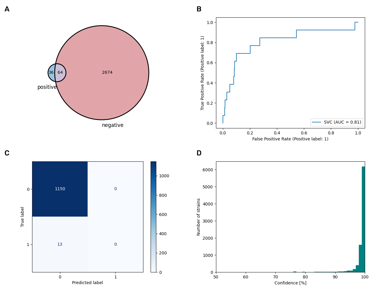
In the following figure is an overview on the model accuracies, the area under the curve (AUC) and the number of new datasets that were added to the database. The acidophile and halophile model failed our quality checks and were thus not integrated into the database (read details below). We show all results of the models in BacDive in a new section called »Genome-based predictions«, but also try to integrate some of the datasets into the respective data fields. We will discuss in the following why it is easier for same data fields and not for others, however, in the last part of the next figure, an overview on these included datasets is shown.
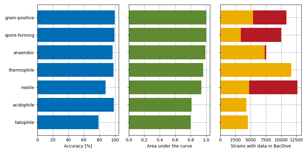
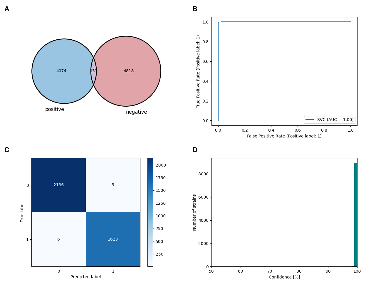
The gram-positive model
The model for Gram staining is well balanced in terms of training data and also very predictive with an accuracy of 99.7%. The database was complemented with 5,500 datasets of Gram staining where no data were previously available.
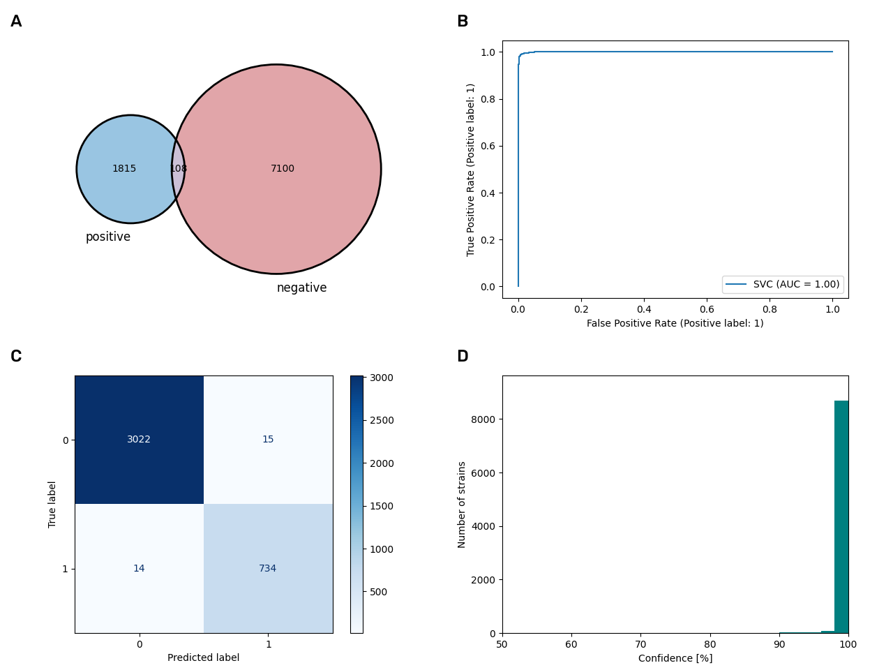
The spore-forming model
Data for the spore-forming model is not so well balanced with 4 times the amount of negative data. However, the model still performs exceedingly good with an accuracy of 99.2% and an area under the curve of 1.00. This model lead to an increase of 6,635 datasets where no information on spore formation was available before.
The anaerobic model
The anaerobic model performs also very well with an accuracy of 97.0% and an AUC of 0.99. However, as
the
BacDive data field for oxygen tolerance covers a number of values besides
anaerobic (e.g.
microaerophilic, facultative aerobic, aerotolerant, etc.) only true predicted data
point could be
added to the database, leading to a total of 257 completely new datasets in BacDive on the
basis of
this model.

The thermophile model
Despite being unbalanced and including a lot of overlapping data (that were of course eliminated from
the
training dataset), the thermophile model performs well with an accuracy of 98.0% and an AUC of 0.96,
resulting
in a high confidence. However, as the figure 1 shows, temperature is one of the most abundant
phenotype data
fields in BacDive. In addition to that, the temperature data field in BacDive covers more
possibilities
than thermophilic or not (e.g. mesophilic, psychrophilic, etc.), meaning that only true
predicted
data could be added to the data fields. This leads to only one dataset that was amended to the
database from
this model.

The motility model
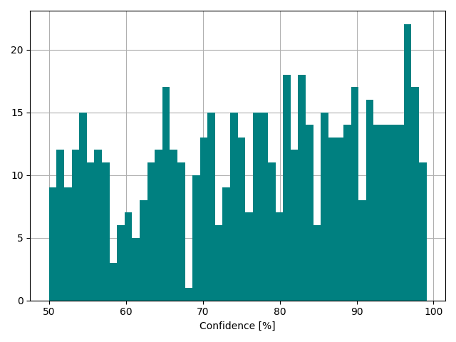
With an accuracy of 88.0% and an AUC of 0.94, the motility model is one of the mid-tier models in this study. The confidence of the predictions is wide-spread among the different strains and the false-positive rate is as high as the false negative rate. As both, positive and negative values can be integrated, this model led to the highest enrichment with new data by adding 7,954 motility datasets.
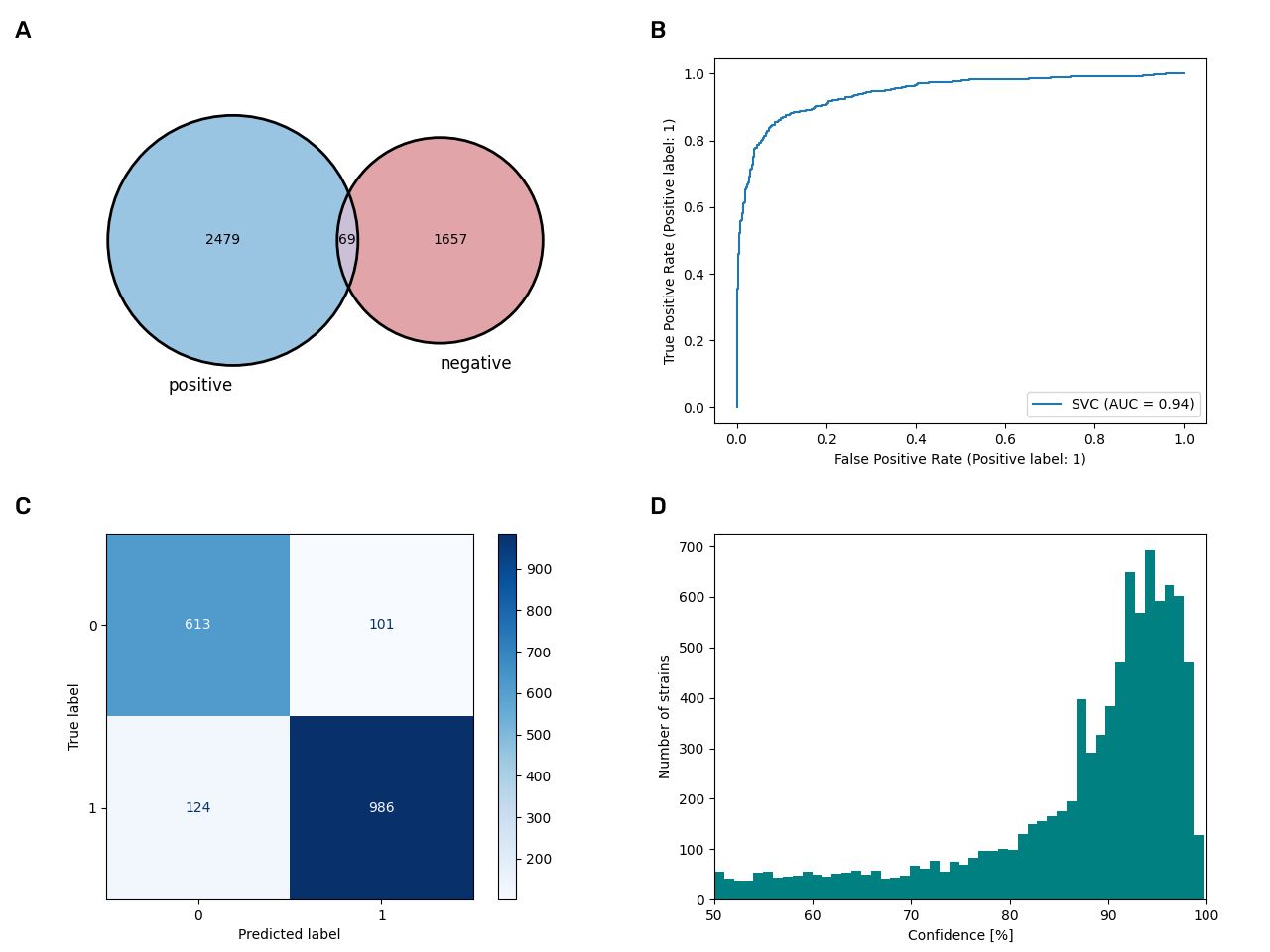
We looked into the question, why the model could predict motility in many cases with high confidence while it fails in other cases. Particularly, we looked into all the datasets were the model failed to predict the manually annotated value. We found 590 instances in the database where the model fails to predict the real data. Among those, 333 are data that were also included in the training dataset, meaning there might be a systematic problem with the data that makes it for a subset of strains not predictable whether they are motile or not. Unfortunately, the prediction confidence mirrors the falsehood of the prediction just to some extent:
The problem likely lies within the fundamentals of motility. In general, bacterial motility can be
divided
into two
principle mechanisms: flagella-based and flagella-independent. The first can include a
number of
different
flagellum arrangements. In contrast, the second contains, among others, gliding that do not depend on
flagella
but instead
on membrane proteins, type IV pili or even polysaccharide jets. As one can imagine, the
difference
between these
types of movement can be pretty hard to predict by one model alone. In BacDive,
information
on the type
of movement is stored in the Flagellum arrangement data field that also
contains
information on
gliding. Unfortunately, this data field contains a large fraction of missing entries (NULL),
as the
following
table depicts.
| Flagellum arrangement | Data sets (total) | Data sets (false) |
|---|---|---|
| NULL | 8973 | 450 |
| gliding | 345 | 121 |
| peritrichous | 243 | 5 |
| polar | 209 | 4 |
| monotrichous, polar | 195 | 7 |
| monotrichous | 39 | 1 |
| lophotrichous | 26 | 2 |
| subpolar | 12 | 0 |
| monopolar | 9 | 0 |
| amphitrichous | 7 | 0 |
| polytrichous, monopolar | 2 | 0 |
When we now have a look at our 590 falsely predicted datasets, we find that more than 20% of them are labeled as gliding and more of 76% do have no value at all, meaning a part of this might also be gliding. In contrast, the model fails to predict known flagellum-based motility only 19 times. Because of this data, we assume that the model especially fails to predict gliding, but might be able to predict flagellum-based motility with an underestimated confidence.
The halophile model
The halophile model has a low accuracy of 78.8% even though the dataset is well balanced. The reason might lies in the way we select the positive and negative data. To distinguish between the two, we take all strains that grow with a minimum of 5.2% NaCl as positive labels and everything with a maximum of 1.7% as negative. Everything in-between is discarded. This might not be the best approach here, since the model might not know how to place in-between datasets correctly, leading to many false predictions. Although this model would gain a total of 2,097 completely new datasets, we decided not to include this data into the BacDive database.

The acidophile model
The acidophile model is a good example for a model that has poor predictive quality despite having an overall good accuracy score. It has an accuracy of 98.4%, but because of a large unbalance in the training data and many overlapping labels, its predictive power is poor. In our experiments, the model was not able to predict any acidophilic strain, but nonetheless received a good score because it was correct in most cases. For this reason, we decided to exclude this model from the integration into BacDive.
Feature importance studies
There are in total 10,752 distinct protein families in the annotated genomes. To reduce the feature dimensions, the families were aggregated into Pfam Clans before training. Pfam Clans are means to cluster structural properties and functional similarities of families. By clustering Pfams into Clans, 542 unique features remain.
The feature importance cannot be derived from the models per se, as non-linear kernels do not support this. The use of a linear kernel, however, leads to a lower accuracy. To avoid this, we tested trained two models independently: one with a linear kernel to extract potential features of importance and a second with a non-linear kernel to do the actual predictions. One has to be aware that the extracted features from the linear model might not be the features that are used for prediction. Instead they should serve as an interpretation guidance by unraveling features that might be of interest.
Interpreting the features, however, might be a it of a challenge as translation of Pfams into Clans might lead to a loss of information. To tackle this challenge, we developed the following approach. First, the most important features were extracted from the linear model (next figure). In general, we took the 10 most important features for both, positive and negative prediction. In the next figure, one can see the feature importance of the Gram-positive model, with Glycosyl transferases (CL0110) as one of the best positive features and outer membrane beta barrels (CL0193) as the best negative feature. However, as the Clan CL0193 contains 117 protein families, interpreting this statement is rather difficult. To address this, we next looked for the most abundant Pfams (in more than 50% of strains) in the dataset that belong to the group of interest (Gram-negative).

To keep a long story short, the best 3 Pfams from the CL0193 Clan were:
- Omp85 superfamily domain: bacterial outer membrane proteins, which can function as protein translocases or as membrane protein assembly factors
- TonB dependent receptors, that are associated with the uptake and transport of large substrates such as iron siderophore complexes and vitamin B12 in gram-negative bacteria
- LPS transport system D, an essential outer membrane protein that mediates the final transport of lipopolysaccharide (LPS) to outer leaflet and is essential for most Gram-negative bacteria
Of course, this result by far not surprising, however, within the CL0401 Clan that has a little lower negative importance is also a highly abundant Protein of unknown function (DUF3971). This study serves as a proof-of-concept to show the significance of feature importance for the study of unknown proteins.